Sandbox Survey: Part 2

Introduction

In the previous lab, small scale, digital elevation models were created in a sandbox. Elevation data was collected for the landscape and compiled into a spreadsheet. The spreadsheet was organized into X,Y, and Z points. This is important because the data needs to be in a coordinate format in order for the DEM to be created. The spreadsheet will be entered into ArcMap and the data will be used to create raster that will depict the elevation. There will be five different interpolation methods used to show the elevation changes in the landscape. 

Methods

The first step to this project was to create a geodatabase to hold all of the elevation rasters, the spreadsheet, and the point feature class that needs to be created. Once the spreadsheet was imported, the point feature class was created. With the newly created point feature class finished and entered into ArcMap, the grid format and the square shape of the landscape can be seen. Figure 1 shows the basic point feature class alone in ArcMap.

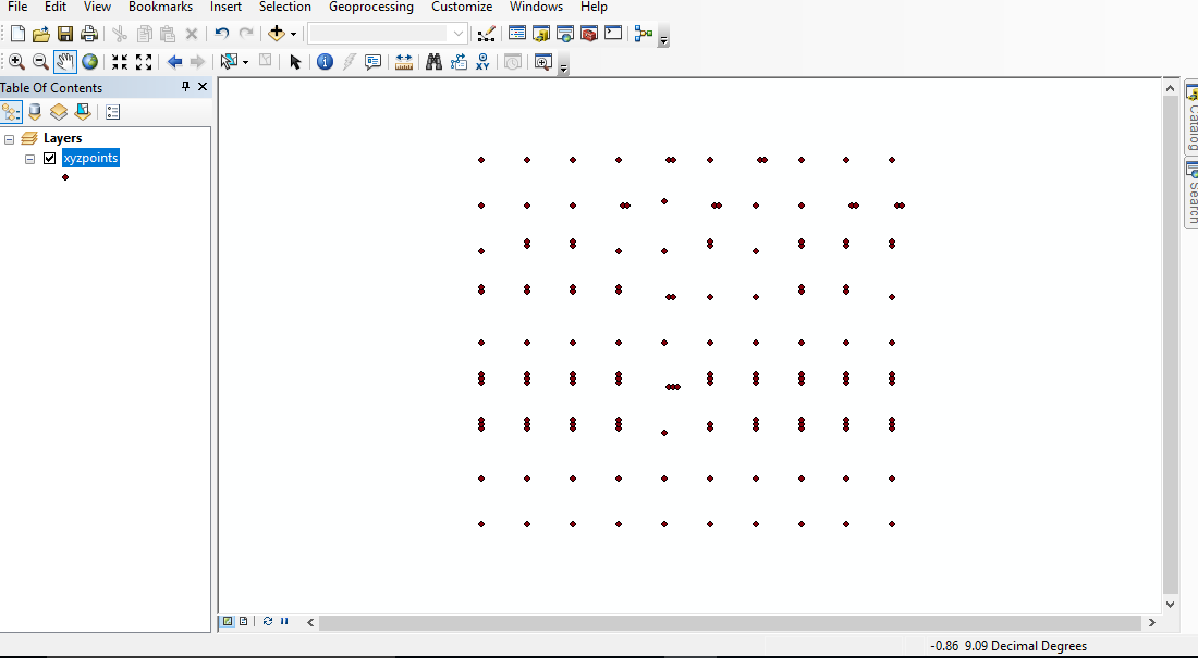Figure 1 is the result of the x,y coordinate plot that was created.

The next step was to use tools in ArcMap in order to create the five different interpolations that were required. The five interpolations that needed to be used were, IDW, Natural Neighbors, Kriging, Spline, and TIN. These interpolation methods are defined below. The definitions come from ArcGIS pro and ArcHelp. 

• IDW (inverse distance weighted technique) assumes that things close to one another are going to be more similar to each other than things further away.
• Natural neighbors makes sure that unsampled areas are similar to one another and never go above or below the min or max sampled points. 
• Kringing is an estimated surface that is generated from a set of scattered points 
• Spline gives a smooth surface by using a mathematical function. This allows for the most pleasing DEM model for this project. 
• TIN (triangulated irregular network) is an assortment of triangles that are given individual values. For the sake of this project, the values are elevation. 

Once each one of the tools that create these interpolations was run, the individual rasters needed to be opened up in ArcScene. The current rasters do not show any elevation change but just assign values to a 2-D image. ArcScene helps to take those values and create a 3-D landscape. This is how each interpolation method can be assessed the best. 

The 3-D images were then exported back into ArcMap so that it was accompanied by its attributes. The orientation of the images is so that the origin point is at the bottom with the y-axis going to the left and the x-axis going to the right. This was the chose orientation because it does the best to show the large ridge in the landscape. 

Results

Figure 2 below, shows all of the final elevation models from each interpolation method that was used. IDW and nearest neighbor interpolation produced a similar result for this project. Both show each data point with some exaggeration and the surrounding area is relatively smooth. Kringling and TIN both provide a rougher "geometric" looking DEM that do a good job showing the elevation change but not realistically depicting the landscape. Spline is the most effective interpolation method for showing a realistic landscape. 

Figure 2 is the compilation of all of the interpolation methods run on the DEM.

When looking back at the survey that was run, there are certain things that could have been changed in order to have more accurate interpolations. The amount of data points collected was, more than likely, not enough. The grid that the measurements were made on was 11x11 which, looking back on it, is not nearly a fine enough resolution. Some of the pixels in the grid were given multiple measurements to show when large elevation changes were happening. The way that these were recorded was not correct. Instead of evenly dividing 1 pixel into tenths of a pixel, the pixel was marked in sections from one to three. This threw off some of the locations of measurements because if it was supposed to be located 1.75 up on the y-axis, it was marked as 1.3. Now having the experience from this project, if it was to be done again, more points would be added and our data collection method would be fixed. All in all, the models do represent the original landscape pretty well but there would be problems if the survey area was larger. 

Conclusion

To summarize the entire two week project, a landscape was created in a sandpit and groups were expected to conduct their own survey of the landscape elevation with fairly minimal instruction. The data that was collected was entered into ArcMap and turned into a digital elevation model using multiple interpolation methods. This project provided a lot of knowledge about how to go about collecting survey data. This was the most in-depth elevation survey project that I have done so unfamiliarity with some of the processes did show in our results. Overall this project provided a learning experience to the very interesting process of elevation surveying.